Application in research

In this example, we will analyze how much the proposition of the European Gas Demand Reduction Plan on 20 July affected Sputnik’s coverage of energy issues in the United States and the European Union.

library(LSX)
#> Warning in .recacheSubclasses(def@className, def, env): undefined subclass
#> "ndiMatrix" of class "replValueSp"; definition not updated
library(quanteda)
#> Package version: 4.0.0
#> Unicode version: 15.1
#> ICU version: 74.1
#> Parallel computing: 16 of 16 threads used.
#> See https://quanteda.io for tutorials and examples.
library(ggplot2)

Preperation

We will analyze the same corpus as the introduction, so too the pre-processing.

corp <- readRDS("data_corpus_sputnik2022.rds") |>
    corpus_reshape()
toks <- tokens(corp, remove_punct = TRUE, remove_symbols = TRUE, 
               remove_numbers = TRUE, remove_url = TRUE)
dfmt <- dfm(toks) |> 
    dfm_remove(stopwords("en"))

We will use a dictionary of keywords in this example.

dict <- dictionary(file = "dictionary.yml")
print(dict[c("country", "energy")])
#> Dictionary object with 2 primary key entries and 2 nested levels.
#> - [country]:
#>   - [us]:
#>     - united states, us, american*, washington
#>   - [uk]:
#>     - united kingdom, uk, british, london
#>   - [eu]:
#>     - european union, eu, european*, brussels
#>   - [se]:
#>     - sweden, swedish, stockholm
#>   - [fi]:
#>     - finland, finnish, helsinki
#>   - [ua]:
#>     - ukraine, ukrainian*, kiev, kyiv
#>   [ reached max_nkey ... 1 more key ]
#> - [energy]:
#>   - gas, oil, engery

Estimate the polarity of words

To measure the sentiment specifically about energy issues, we collect words that occur frequently around keywords such as “oil”, “gas”, “energy” and passing them to terms. These keywords are called target words.

seed <- as.seedwords(data_dictionary_sentiment)
term <- char_context(toks, pattern = dict$energy, p = 0.01)
lss <- textmodel_lss(dfmt, seeds = seed, terms = term, cache = TRUE, 
                     include_data = TRUE, group_data = TRUE)

textplot_terms(lss, highlighted = data_dictionary_LSD2015[1:2])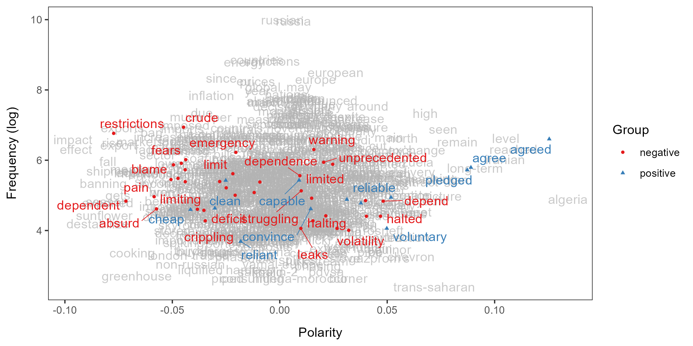

Predict the polarity of documents

We can extract the document variables from the DFM in the LSS model and save the predicted polarity scores as a new variable.

dat <- docvars(lss$data)
dat$lss <- predict(lss)
print(nrow(dat))
#> [1] 8063

Detect the mentions of country/region

We can detect the mentions of countries using the dictionary. If you want to classify texts by country more accurately, you should use the newsmap package.

dfmt_dict <- dfm(tokens_lookup(toks, dict$country[c("us", "eu")]))
print(head(dfmt_dict))
#> Document-feature matrix of: 6 documents, 2 features (91.67% sparse) and 4 docvars.
#>                features
#> docs            us eu
#>   s1092644731.1  2  0
#>   s1092644731.2  0  0
#>   s1092644731.3  0  0
#>   s1092644731.4  0  0
#>   s1092644731.5  0  0
#>   s1092644731.6  0  0

We can create dummy variables for mentions of country/region by dfm_group(dfmt_dict) > 0. We must group documents because the unit of analysis is the articles in this example (recall textmodel_lss(group_data = TRUE) above).

mat <- as.matrix(dfm_group(dfmt_dict) > 0)
print(head(mat))
#>              features
#> docs             us    eu
#>   s1092644731  TRUE FALSE
#>   s1092643478  TRUE  TRUE
#>   s1092643372 FALSE FALSE
#>   s1092643164  TRUE FALSE
#>   s1092641413  TRUE FALSE
#>   s1092640142  TRUE FALSE
dat <- cbind(dat, mat)

Results

We must smooth the polarity scores of documents separately for the country/region using smooth_lss(). After smoothing, we can see that the difference between the US and EU has expanded soon after the proposition of the European Gas Demand Reduction Plan.

smo_us <- smooth_lss(subset(dat, us), lss_var = "lss", date_var = "date")
smo_us$country <- "us"
smo_eu <- smooth_lss(subset(dat, eu), lss_var = "lss", date_var = "date")
smo_eu$country <- "eu"
smo <- rbind(smo_us, smo_eu)

ggplot(smo, aes(x = date, y = fit, color = country)) + 
    geom_line() +
    geom_ribbon(aes(ymin = fit - se.fit * 1.96, ymax = fit + se.fit * 1.96, fill = country), 
                alpha = 0.1, colour = NA) +
    geom_vline(xintercept = as.Date("2022-06-26"), linetype = "dotted") +
    scale_x_date(date_breaks = "months", date_labels = "%b") +
    labs(title = "Sentiment on energy", x = "Date", y = "Sentiment", 
         fill = "Country", color = "Country")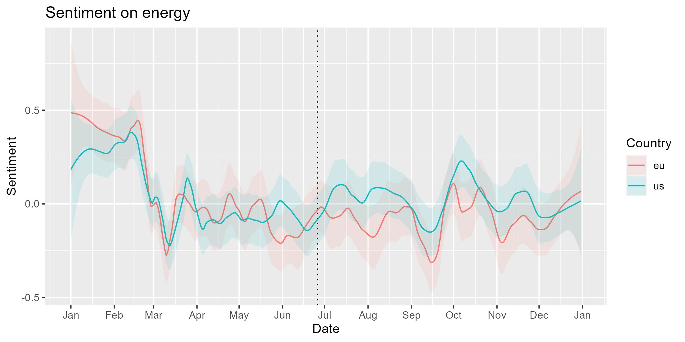

To test if the changes after the proposition is statistically significant, we should create a dummy variable after for the period after the proposition and perform regression analysis with its interactions with the country/region dummies. This is akin to the difference-in-differences design that I often employ in analysis of news (Watanabe 2017; Watanabe et al. 2022).

dat_war <- subset(dat, date >= as.Date("2022-02-24"))
dat_war$after <- dat_war$date >= as.Date("2022-06-20")
summary(dat_war[c("lss", "us", "eu", "after")])
#>       lss               us              eu            after        
#>  Min.   :-9.65775   Mode :logical   Mode :logical   Mode :logical  
#>  1st Qu.:-0.64778   FALSE:2450      FALSE:4547      FALSE:3394     
#>  Median :-0.03249   TRUE :4696      TRUE :2599      TRUE :3752     
#>  Mean   :-0.03571                                                  
#>  3rd Qu.: 0.53997                                                  
#>  Max.   : 7.59192                                                  
#>  NA's   :4

dat_war contains only the scores since the beginning of the war, so the intercept is the average sentiment of the articles without the mentions of the US or the EU before the proposition during the war; usTRUE and euTRUE are the average sentiment for the articles with the mentions of the US and the EU in the period, respectively.

The coefficient of afterTRUE indicates that the overall sentiment became more negative after the proposition (β = -0.11; p < 0.01). The insignificant coefficient of euTRUE:afterTRUE shows that the sentiment for the EU also decreased, but the large positive coefficient of usTRUE:afterTRUE suggests that the sentiment for the US increased (β = 0.22; p < 0.001) and became more positive than before the proposition.

reg <- lm(lss ~ us + eu + after + us * after + eu * after, dat_war)
summary(reg) 
#> 
#> Call:
#> lm(formula = lss ~ us + eu + after + us * after + eu * after, 
#>     data = dat_war)
#> 
#> Residuals:
#>     Min      1Q  Median      3Q     Max 
#> -9.6176 -0.6074  0.0021  0.5784  7.5495 
#> 
#> Coefficients:
#>                  Estimate Std. Error t value Pr(>|t|)    
#> (Intercept)       0.03147    0.03223   0.977  0.32880    
#> usTRUE           -0.07167    0.03728  -1.923  0.05457 .  
#> euTRUE           -0.04580    0.03652  -1.254  0.20979    
#> afterTRUE        -0.13860    0.04372  -3.170  0.00153 ** 
#> usTRUE:afterTRUE  0.22118    0.05048   4.382 1.19e-05 ***
#> euTRUE:afterTRUE -0.02027    0.04972  -0.408  0.68346    
#> ---
#> Signif. codes:  0 '***' 0.001 '**' 0.01 '*' 0.05 '.' 0.1 ' ' 1
#> 
#> Residual standard error: 1.004 on 7136 degrees of freedom
#>   (4 observations deleted due to missingness)
#> Multiple R-squared:  0.00394,    Adjusted R-squared:  0.003242 
#> F-statistic: 5.645 on 5 and 7136 DF,  p-value: 3.362e-05

Conclusions

Our analysis shows that the Sputnik covered the energy issues in the US more positively while those in the EU more negatively after the proposition the European Gas Demand Reduction Plan. Our findings are preliminary, but we can give them a tentative interpretation: the Russian government attempted to create divisions between the US and the EU by emphasizing the different impact of the Ukraine war and the sanctions against Russia on American and European lives.

References

Watanabe, K. (2017). Measuring news bias: Russia’s official news agency ITAR-TASS’ coverage of the Ukraine crisis. European Journal of Communication. https://doi.org/10.1177/0267323117695735.
Watanabe, K., Segev, E., & Tago, A. (2022). Discursive diversion: Manipulation of nuclear threats by the conservative leaders in Japan and Israel, International Communication Gazette. https://doi.org/10.1177/17480485221097967.